In this post I would like to compare some fundamental characteristics of two platforms for scientific computations: Matlab from Mathworks and Python with dedicated libraries. A simple program for calculation of spectrum of a signal should be appropriate for comparison of basic features of both languages, similarities and differences in their syntax, ease of implementing, and clarity of the code.
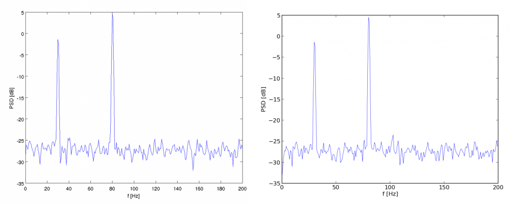
Presented Matlab script calculates power spectral density of the simulated signal, containing two oscillatory components at frequencies 30 and 80 Hz. The spetrum is calculated by hand, by means of fast Fourier transform function, windowing is made with Hanning window.
tic fs=400; T=10; nfft=512; overlap=0.5; A1=1; f1=30; fi1=0; A2=2; f2=80; fi2=2; An=1.5; t=0:1/fs:T; t=t(:); % make 't' a column vector sig=A1*cos(2*pi*f1*t+fi1) + A2*cos(2*pi*f2*t+fi2); noise=An*rand(length(t),1); x=sig+noise; wind=hanning(nfft); noverlap=fix(nfft*overlap); nadvance=nfft-noverlap; nrecs=fix((length(t)-noverlap)/nadvance); Pxx=zeros(nfft,1); ind=1:nfft; for k=1:nrecs xs=x(ind); xs=(xs(:)-mean(xs)).*wind; Xf=fft(xs,nfft)/nfft; Pxx=Pxx+abs(Xf).^2; ind=ind+nadvance; end Pxx=Pxx(1:nfft/2); f=(0:nfft/2-1)/(nfft/2-1)*(fs/2); figure plot(f,10*log10(Pxx)) % in dB xlabel('f [Hz]') ylabel('PSD [dB]') saveas(gcf,'fig_PSD_matlab.png','png') % time czas=toc; czas_=['Time: ' int2str(fix(czas/3600)) ' hours, ' ... int2str(fix(czas/60)-fix(czas/3600)*60) ' min and ' ... num2str(mod(czas,60),'%0.2f') ' s.']; disp(' '); disp(czas_) |
The same program written in Python language, using NumPy and Matplotlib libraries would look like this:
import numpy, pylab, time from math import pi tic=time.clock() fs,T=400,10 nfft=512 overlap=0.5 A1,f1,fi1 = 1,30,0 A2,f2,fi2 = 2,80,2 An=1.5 t=numpy.arange(0,T,1./fs) t=t.transpose() sig=A1*numpy.cos(2*pi*f1*t+fi1) + A2*numpy.cos(2*pi*f2*t+fi2) noise=An*numpy.random.rand(len(t)) x=sig+noise wind=numpy.hanning(nfft) noverlap=numpy.fix(nfft * overlap) nadvance=nfft-noverlap nrecs=numpy.fix((len(t)-noverlap)/nadvance) Pxx=numpy.zeros((nfft)) ind=numpy.arange(0,nfft,1) for k in range(nrecs): xs=x[ind] xs=numpy.multiply((xs-numpy.mean(xs)),wind) Xf=numpy.fft.fft(xs,nfft)/nfft Pxx=Pxx+numpy.square(numpy.abs(Xf)) ind=ind+int(nadvance) Pxx=Pxx[0:nfft/2] f=numpy.arange(0.0,nfft/2,1)/(nfft/2-1)*(fs/2) pylab.figure pylab.plot(f,10*numpy.log10(Pxx),linewidth=0.5) # in dB pylab.xlabel('f [Hz]') pylab.ylabel('PSD [dB]') pylab.savefig("fig_PSD_python.png") pylab.show() # time toc = time.clock() czas=toc - tic czas_='Time: ' czas_=czas_ + "%0.*f" %(0,numpy.fix(czas/3600)) + ' hours, ' czas_=czas_ + "%0.*f" %(0,numpy.fix(czas/60)-numpy.fix(czas/3600)*60) + ' min and ' czas_=czas_ + "%0.*f" %(2,numpy.mod(czas,60)) + ' s.' print(czas_) |
At first glance, big similarity between two programs can be seen and it seems that it should be relatively easy for Matlab user to start working with Python, making use of dedicated libraries. Both languages are of high level, and allow for a wide variety of possible solutions of the problem. Libraries for numerical computation contain functions with similar names, arguments and giving similar results to the functions that Matlab users sre familiar with. Nevertheless, after few years of working with Matlab, there are some elements, that I got used to, that Python lacks. For example there are no dot operators explicitly marking element wise operations on the tables, or clean and simple matrix notation in the form: a=[1,2,3;4,5,6].
The figure presents results of using Matlab plot() function (left) and its equivalent function from the Matplotlib library (right).
Approximated time of the execution of these both programs is similar. On a laptop computer with Intel Core 2 Duo 2 GHz processor:
Matlab: 0.25 s [0.24-0.26]
Python: 0.26 s [0.25-0.27]
I found it interesting that for Matlab script executed in Octave it took signifficantly less time to do these calculations:
Octave: 0.08 s [0.07-0.09]
In order to compare performance of both environments, more calculations should be done. In next article I will present results of such a comparison, using programs requiring much more computational power.

 English


 polski