Skip to content

Archive

Category: Biomedical Physics

Criteria for detection of transiently evoked otoacoustic emissions in schoolchildren
Bartosz Trzaskowski, Edyta Pilka, W. Wiktor Jedrzejczak, Henryk Skarzynski
International Journal of Pediatric Otorhinolaryngology 79 (2015), pp. 1455-1461
http://www.sciencedirect.com/science/article/pii/S0165587615003043

Objectives
The aim was to compare, on the same dataset, existing detection criteria for transiently evoked otoacoustic emissions (TEOAEs) and to select those most suitable for use with school-aged children.

Methods
TEOAEs were recorded from the ears of 187 schoolchildren (age 8–10 years) using the Otodynamics ILO 292 system with a standard click stimulus of 80 dB peSPL. Pure tone audiometry and tympanometry were also conducted. Global and half-octave-band (at 1, 1.4, 2, 2.8, 4 kHz) values of OAE signal-to-noise ratio (SNR), reproducibility, and response level were determined. These parameters were used as criteria for detection of TEOAEs. In total, 21 criteria based on the literature and 3 new ones suggested by the authors were investigated.

Results
Pure tone audiometry and tympanometry screening generated an ear-based failure rate of 7.49%. For TEOAEs, there was a huge variability in failure rate depending on the criteria used. However, three criteria sets produced simultaneous values of sensitivity and specificity above 75%. The first of these criteria was based only on a global reproducibility threshold value above 50%; the second on certain global reproducibility and global response values; and the third involved exceeding a threshold of 50% band reproducibility. The two criteria sets with the best sensitivity were based on global reproducibility, response level, and signal-to-noise ratio (with different thresholds across frequency bands).

Conclusions
TEAOEs can be efficiently used to test the hearing of schoolchildren provided appropriate protocols and criteria sets are used. They are quick, repeatable, and simple to perform, even for nonaudiologically trained personnel. Criteria with high sensitivity (89%) were identified, but they had relatively high referral rates. This is not so much a problem in schoolchildren as it is in newborns because with schoolchildren pure tone audiometry and tympanometry can be performed immediately or at a follow-up session. Nevertheless, high referral rates lead to increased screening cost; for that reason, three less rigorous criteria with high values of both sensitivity and specificity (75% and above) are recommended.

Comparison of wave V detection algorithms in auditory brainstem responses.
Bartosz Trzaskowski
Nowa Audiofonologia 2015; 4(2):43-52

In this paper, selected systems of automatic ABR detection described in scientific journals by different research teams were presented and compared.

Otoacoustic Emissions before and after Listening to Music on a Personal Player
Bartosz Trzaskowski, W. Wiktor Jędrzejczak, Edyta Piłka, Magdalena Cieślicka, Henryk Skarżyński
Med Sci Monit 2014; 20:1426-1431
http://www.medscimonit.com/abstract/index/idArt/890747

The main aim of this study was to investigate whether listening to music on a CD player affects parameters of otoacoustic emissions. A group of 20 adults with normal hearing were tested. No statistically significant changes in either OAE parameters or PTA thresholds were found.

New paper published in Otorynolarynglogia presenting results of evaluation of system for automatic detection of auditory brainstem responses

System for automatic detection of auditory brainstem responses. II. Evaluation of the system for clinical data.
Bartosz Trzaskowski, Krzysztof Kochanek, W. Wiktor Jędrzejczak, Adam Piłka, Henryk Skarżyński
Otorynolaryngologia, 2013; 12(4): 183-189
http://www.mediton.pl/PL/czasopisma/otorynolaryngologia/archiwum_12.4.0.html

New paper published in Otorynolaryngologia:

System for automatic detection of auditory brainstem responses. I. Characteristics and tests.
Bartosz Trzaskowski, W. Wiktor Jedrzejczak, Edyta Pilka, Krzysztof Kochanek, Henryk Skarzynski
Otorynolaryngologia, 2013; 12(3): 137-147
http://www.mediton.pl/PL/czasopisma/otorynolaryngologia/archiwum_12.3.0.html

A new paper presenting system for automatic detection and removal of sonomotor waves from auditory brainstem responses (ABR) has been published in Computers in Biology and Medicine

Automatic removal of sonomotor waves from auditory brainstem responses

In this paper, a computerized technique for automatic detection and removal of sonomotor waves (SMWs) from auditory brainstem responses (ABRs) was proposed. The method was based on adaptive decomposition using a redundant set of Gaussian and 1-cycle-limited Gabor functions. Its efficiency was tested by means of simulated and clinical data. Obtained results were good and confirmed by an expert.

In this post I would like to compare some fundamental characteristics of two platforms for scientific computations: Matlab from Mathworks and Python with dedicated libraries. A simple program for calculation of spectrum of a signal should be appropriate for comparison of basic features of both languages, similarities and differences in their syntax, ease of implementing, and clarity of the code.

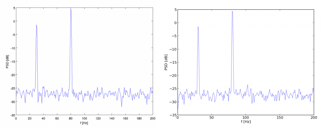
Presented Matlab script calculates power spectral density of the simulated signal, containing two oscillatory components at frequencies 30 and 80 Hz. The spetrum is calculated by hand, by means of fast Fourier transform function, windowing is made with Hanning window.

tic
 
fs=400; T=10;
 
nfft=512;
overlap=0.5;
 
A1=1; f1=30; fi1=0;
A2=2; f2=80; fi2=2;
An=1.5;
 
t=0:1/fs:T;
t=t(:); % make 't' a column vector
 
sig=A1*cos(2*pi*f1*t+fi1) + A2*cos(2*pi*f2*t+fi2);
noise=An*rand(length(t),1);
 
x=sig+noise;
 
wind=hanning(nfft);
 
noverlap=fix(nfft*overlap);
nadvance=nfft-noverlap;
nrecs=fix((length(t)-noverlap)/nadvance);
 
Pxx=zeros(nfft,1);
ind=1:nfft;
for k=1:nrecs
    xs=x(ind);
    xs=(xs(:)-mean(xs)).*wind;
    Xf=fft(xs,nfft)/nfft;
    Pxx=Pxx+abs(Xf).^2;
    ind=ind+nadvance;
end
 
Pxx=Pxx(1:nfft/2);
f=(0:nfft/2-1)/(nfft/2-1)*(fs/2);
 
figure
plot(f,10*log10(Pxx)) % in dB
xlabel('f [Hz]')
ylabel('PSD [dB]')
saveas(gcf,'fig_PSD_matlab.png','png')
 
% time
czas=toc;
czas_=['Time: ' int2str(fix(czas/3600)) ' hours, ' ...
    int2str(fix(czas/60)-fix(czas/3600)*60) ' min and ' ...
    num2str(mod(czas,60),'%0.2f') ' s.'];
disp(' ');
disp(czas_)

The same program written in Python language, using NumPy and Matplotlib libraries would look like this:

import numpy, pylab, time
from math import pi
 
tic=time.clock()
 
fs,T=400,10 
 
nfft=512
overlap=0.5
 
A1,f1,fi1 = 1,30,0 
A2,f2,fi2 = 2,80,2 
An=1.5
 
t=numpy.arange(0,T,1./fs)
t=t.transpose()
 
sig=A1*numpy.cos(2*pi*f1*t+fi1) + A2*numpy.cos(2*pi*f2*t+fi2)
noise=An*numpy.random.rand(len(t))
x=sig+noise
 
wind=numpy.hanning(nfft)
 
noverlap=numpy.fix(nfft * overlap)
nadvance=nfft-noverlap
nrecs=numpy.fix((len(t)-noverlap)/nadvance)
 
Pxx=numpy.zeros((nfft))
ind=numpy.arange(0,nfft,1)
for k in range(nrecs):
    xs=x[ind]
    xs=numpy.multiply((xs-numpy.mean(xs)),wind)
    Xf=numpy.fft.fft(xs,nfft)/nfft
    Pxx=Pxx+numpy.square(numpy.abs(Xf))
    ind=ind+int(nadvance)
 
Pxx=Pxx[0:nfft/2]
f=numpy.arange(0.0,nfft/2,1)/(nfft/2-1)*(fs/2)
 
pylab.figure
pylab.plot(f,10*numpy.log10(Pxx),linewidth=0.5) # in dB
pylab.xlabel('f [Hz]')
pylab.ylabel('PSD [dB]')
pylab.savefig("fig_PSD_python.png")  
pylab.show()
 
# time
toc = time.clock()
czas=toc - tic
czas_='Time: '
czas_=czas_ + "%0.*f" %(0,numpy.fix(czas/3600)) + ' hours, '
czas_=czas_ + "%0.*f" %(0,numpy.fix(czas/60)-numpy.fix(czas/3600)*60) + ' min and '
czas_=czas_ + "%0.*f" %(2,numpy.mod(czas,60)) + ' s.'
print(czas_)

At first glance, big similarity between two programs can be seen and it seems that it should be relatively easy for Matlab user to start working with Python, making use of dedicated libraries. Both languages are of high level, and allow for a wide variety of possible solutions of the problem. Libraries for numerical computation contain functions with similar names, arguments and giving similar results to the functions that Matlab users sre familiar with. Nevertheless, after few years of working with Matlab, there are some elements, that I got used to, that Python lacks. For example there are no dot operators explicitly marking element wise operations on the tables, or clean and simple matrix notation in the form: a=[1,2,3;4,5,6].

The figure presents results of using Matlab plot() function (left) and its equivalent function from the Matplotlib library (right).

Approximated time of the execution of these both programs is similar. On a laptop computer with Intel Core 2 Duo 2 GHz processor:
Matlab: 0.25 s [0.24-0.26]
Python: 0.26 s [0.25-0.27]

I found it interesting that for Matlab script executed in Octave it took signifficantly less time to do these calculations:
Octave: 0.08 s [0.07-0.09]

In order to compare performance of both environments, more calculations should be done. In next article I will present results of such a comparison, using programs requiring much more computational power.

Recently, the number of people, using Python for numerical computation is increasing. I also started to think of migrating some of my scientific work from Matlab to Python. There are some arguments in favor of Python.

First of all it is free. In comparison to Matlab it is a major upside, because the price of just basic Matlab is significant, and purchase of optional toolboxes, further increase total cost of the Mathworks solution. Free Python libraries like: NumPy, SciPy, Matplotlib or IPython, deliver most of the functionality of basic Matlab installation and some functionality of additional toolboxes.

Second, Python is a programming language with interpreters available for almost all platforms. In many systems it is delivered together with the distribution by default. Because of that, it is possible (after installing required libraries) to execute programs written in Python on almost every computer. On the other hand, mainly because of its price, Matlab is most often purchased by scientific institutions, universities or big companies. And mostly with the license restricted to small number of stations or concurrent sessions. Because of that reason, programs written in Matlab can be only executed by people having access to this platform, usually at their work or in school. In this place it should be mentioned, that there is a free alternative to Matlab – Octave. It’s syntax is almost identical to Matlab’s, and any differences in syntax and behavior of functions are considered bugs and they are being fixed. But these two platforms are still not 100% compatible with each other [Porting programs from Matlab to Octave], and even if most of the simple programs in Matlab can be run in Octave, there can be some problems to execute the more complicated ones. Simple Matlab scripts published on this website should execute in Octave 3.2.4 or higher with no errors. There should be no problems with execution of Python scripts (after installation of necessary libraries).

Another upside of Python: it is a full programming language, not an environment dedicated to numerical computations. Because of that, it is easier to use Python for operations not strictly related to computations, when necessary. Large number of dedicated libraries, optimized to specific tasks greatly simplifies the implementation. Python can be used as a scripting language for automation of repeating tasks, and simultaneously, after importing of required libraries, it can be used to perform scientific computations. Many applications has their API in Python. I can easily imagine a situation, where in order to make use of one of my earlier programs in such an application, I just copy with no changes functions and pieces of my Python code. Scripts written in Matlab are useless in this case.

To be fair, there are quite a few upsides of Mathwoks environment also. Matlab is one of the most commonly used platform for computations in the world. It has been used by scientists in many areas for years, and it is a standard in universities. Calculations for scientific publications are performed mostly in Matlab, and blocks of code and algorithms are published in Matlab language. Just because of that it pays off to be familiar with Matlab syntax.

Another advantage of Mathworks platform over Python is, that it delivers one, complete, simple to install environment, having all elements required to work in one place. Right after installation, including automatic installation of purchased toolboxes, the user can run one, complete environment containing: command window, integrated editor, overview of variables in workspaces, debugger, profiler, command history, file browser, on-line help, and even access to internet databases of scripts shared by Matlab community. Workflow is simplified by import and export wizards for common file formats, clipboard data handling or integrated tools for figure manipulation. In my opinion it is a really big Matlab upside, that right after a simple installation user gets complete environment containing many tools simplifying workflow.

Another important upside of Mathwork product is Simulink – environment for simulations and design, integrated with Matlab. Optional dedicated toolboxes can also be purchased for Simulink. Simulink together with Matlab is a powerful platform capable of analysis of dynamic systems behavior, visualization of simulations, data modeling and many others. Currently there is no really concurrent software for Simulink, offering similar capabilities.

There are many pages on the web, comparing Matlab and Python and their pros and cons in different applications. Arguments listed here, pros and cons for each of the two environments are my subjective opinion. I pointed the differences, which I considered significant in my applications – computations in the area of digital signal processing. Other people can have different judgments, based on their own preferences and expectations. In order to evaluate practical aspects of work with these two languages, I would like to perform some computations in both, comparing ease of implementation, execution times etc. As I have no big experience in programming with Python, and on the other hand I would like to do something more interesting than printing some numbers in a loop, I will publish in next posts the examples of usage of both languages to do some simple cases of simulated signals, sound and image processing.

MS Windows users, can download binary versions of many scientific Python libraries on the page: Unofficial Windows Binaries for Python Extension Packages, maintained by Christoph Gohlke. For Linux systems users, it will be easier to use libraries from official repositories or compile the most recent versions from sources.

At the end, links to two open source computation systems: Scilab and SAGE.
In the journal Acta Bio-Optica et Informatica Medica Inżynieria Biomedyczna after long waiting, paper Application of the system of automatic detection and removal of sonomotor wave from auditory brainstem responses has been published.

This paper describes early version of the system. More sophisticated version of the algorithm has been send to another international journal and at the moment it is waiting for a review.