In the previous post I presented the response function of Nikon D70 saving images in JPG Fine format. In this article I would like to show what is the response function for this camera while saving images as NEF, which is the native format of Nikon to record raw data (RAW). Images in this format are essentially unprocessed recordings of data that was registered on a camera sensor. As unprocessed I mean, in this case, the lack of camera postprocessing such as gamma conversion, or white balance. However, processing of the data registered by the sensor already starts during the digitization. That is analog to digital conversion of the analog information from the sensor (in a form of charge) to the information in a discrete digital form. Such a quantization of continuos values is associated with processing of the information. But as some inquisitive users reported, Nikon is messing and changing recorded information already at this stage.
In particular, it has been proved, that recording of images in NEF with lossless compression format used in Nikon D70, is lossy, which is in oposition to the information given by the manufacturer. For the most part, the loss of information is associated with lowering the resolution in the highlights. The Nikon D70 is equipped with Sony ICX413AQ sensor and 12-bit analog-to-digital convertor. 12-bit resolution allows to record 2^12=4096 levels of brightness. But when converting to RAW, the number of levels is limited to 683 and after that, the stripped data are passed to perform lossless compression on them, similar to those used in ZIP files. While lossless compression is lossless indeed, the information is lost at the stage of quantization to 683 discrete brightness value. Quantization curve is saved in NEF files. This encoding preserves the full dynamic range, but conversion of 12-bit information (4096 levels ) into 683 discrete values causes the decrease of resolution in brightness. The shape of the quantization curve, which starts linear and and then increases quadratically, results in lowering the resolution while increasing brightness. Probably, the purpose of this type of conversion was to gain a significant speed up (almost an order of magnitude) during in-camera processing and recording of NEF files. Older models (such as the D1H and D100) were able to process the image even for 20-30 seconds performing compression before saving. Nowadays some of the recent camera models allow to select the recording mode of NEF files: 12 or 14-bit formats, and compressed or uncompressed files.
Additionally, some loss of information in D70 is related to use of the optical low-pass filter designed to remove high-frequency components from the image. Camera sensor when capturing the scene as is actually sampling it with a certain frequency called the sampling rate. However, if the scene contains frequencies higher than half of the sampling frequency, then in the recorded image aliasing will occure, which is known to photographers or graphic artists as moiré effect. To counteract this phenomenon, the digital camera manufacturers have been placing a blurring filter in front of a sensor for many years. This solution ensured that frequencies higher than acceptable for a given sensor will be filtered out, and the sensor will capture only the allowed frequencies. It is also easy to guess what is the relation between sampling frequency and the size of the matrix (in megapixels). The larger the size in MPx, the higher the sampling rate, and the higher frequencies can be recorded by a given sensor without risk that aliasing effect will occure. Recently, due to technological advances and the continuing growth of the size of recorded images, a tendency to remove this filter can be observed, which has a positive impact on improving the focus and increase the detail of the photos. Even Nikon removed the optical low-pass filter from its latest model D5300, assuming that the problem of moiré is not so importantthe with the images with size of 24 MPx.
However, despite the above-mentioned transformations, one would expect that, because the camera did not perform gamma compression (as in the case of JPG files), and the sensor in Nikon D70 is a CCD (with the charge proportional to the exposure) that the dependence of response here may be close to linear. I decided to investigate the relation so I performed the calculations presented below.
I analyzed two series of photos taken with different exposures. The photos were taken exactly as I described in a previous article, with one difference, that this time they have been saved in NEF format. Actually, they were exactly the same scenes photographed under the same conditions because series of NEFs were taken immediately before series of JPGs.
Both series of photos in NEF format look like this:

Barckets. Series 1. NEF.
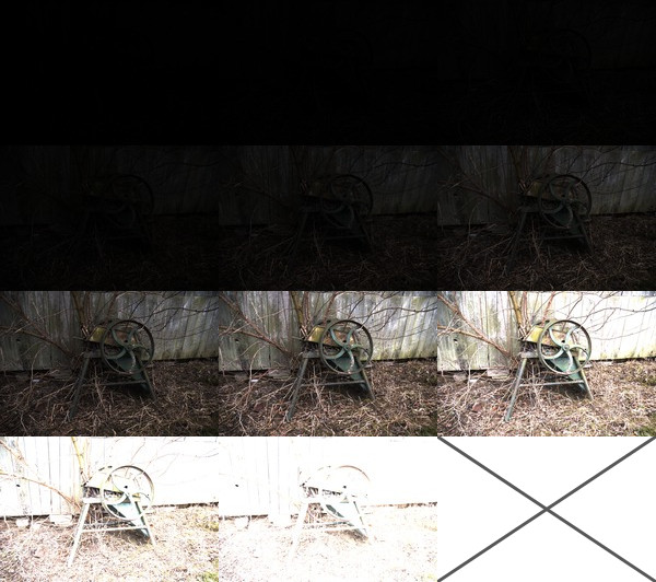
Barckets. Series 2. NEF.
It is easy to notice that, for both series, pictures in NEF format look much darker and with more contrast than pictures in JPG format. It is so because the images in NEF format are in linear color space and images in JPG format in logarythmic. Our visual system, just like all our senses, naturally works in logarythmic way. Images presented in logarythmic color space (like for example taken with conventional film photography) seem much natural and photorealistic to us. That is why, before recording images in a final form of JPGs, the camera compressed them to logarythmic color space using power law transformation – so called gamma conversion. This caused much more natural to us distribution of pixel values in the pictures.
The actual bit resolution of Nikon D70 NEF files is: log2(683)=9.42 bits. In order to perform the calculations, I transformed NEF files into 8 -bit TIFF files. For this purpose, I used a program: dcraw written by Dave Coffin. Conversion could not introduce any automatic changes to brightness (by default dcraw stretches the histogram in such a way that 1% of the pixels is displayed as white), it should not perform gamma conversion, or pixel resampling, neither change the color space of the image. The command I used was “dcraw -T -W -g 1 1 -v -j -o 0”. NEF images captured by Nikon D70 are 3039×2014 px. The mask to select pixels for calculations, was created the same way as in the case of JPG images – as a table 30×20 px evenly spaced in the image while maintaining a 5% margin from the edge of the image.
In order to properly estimate a response curve for 14-bit NEF files, for a series of 11 exposures, with this method, according to the relationship : N*(P-1)>(Zmax-Zmin), one would need to use: N>(2^14-1)/(11-1), which is at least 1639 pixels. A matrix for a system of linear equations would occupy: (1639*11+2^14+1)*(2^14+1639)*16/1000/1000/1000=9.9GB of RAM. Of course, the function proposed by Debevec and Malik also would have to be modified to take account of the 14-bit resolution: Zmax=2^14-1 and shifting the distribution to the brightness of Z=(2^14)/2-1.
Response curves for NEF files with Nikon D70:
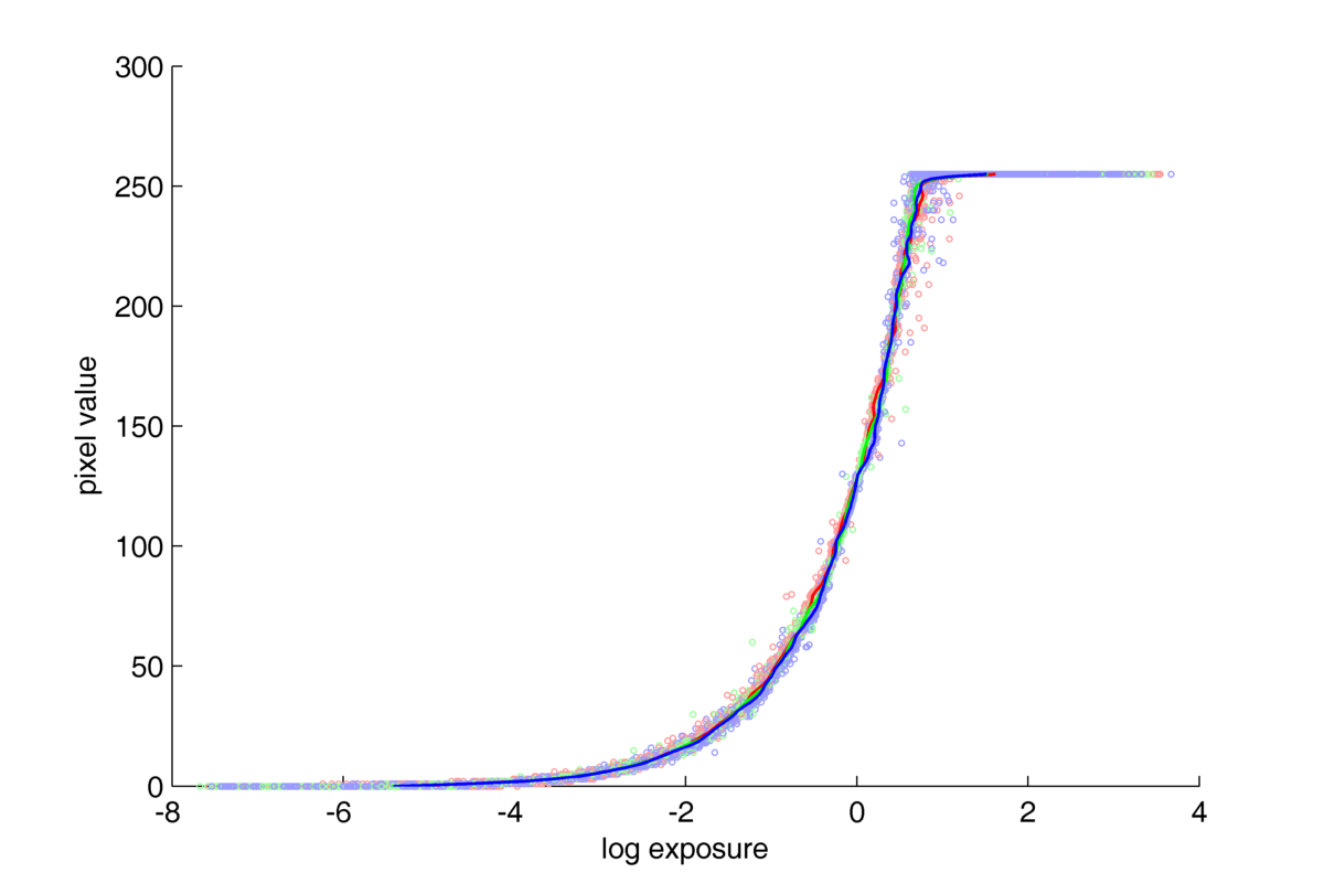
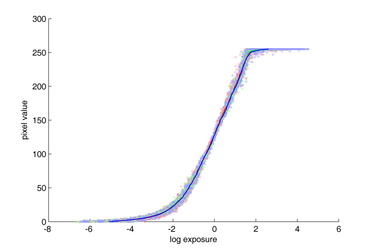
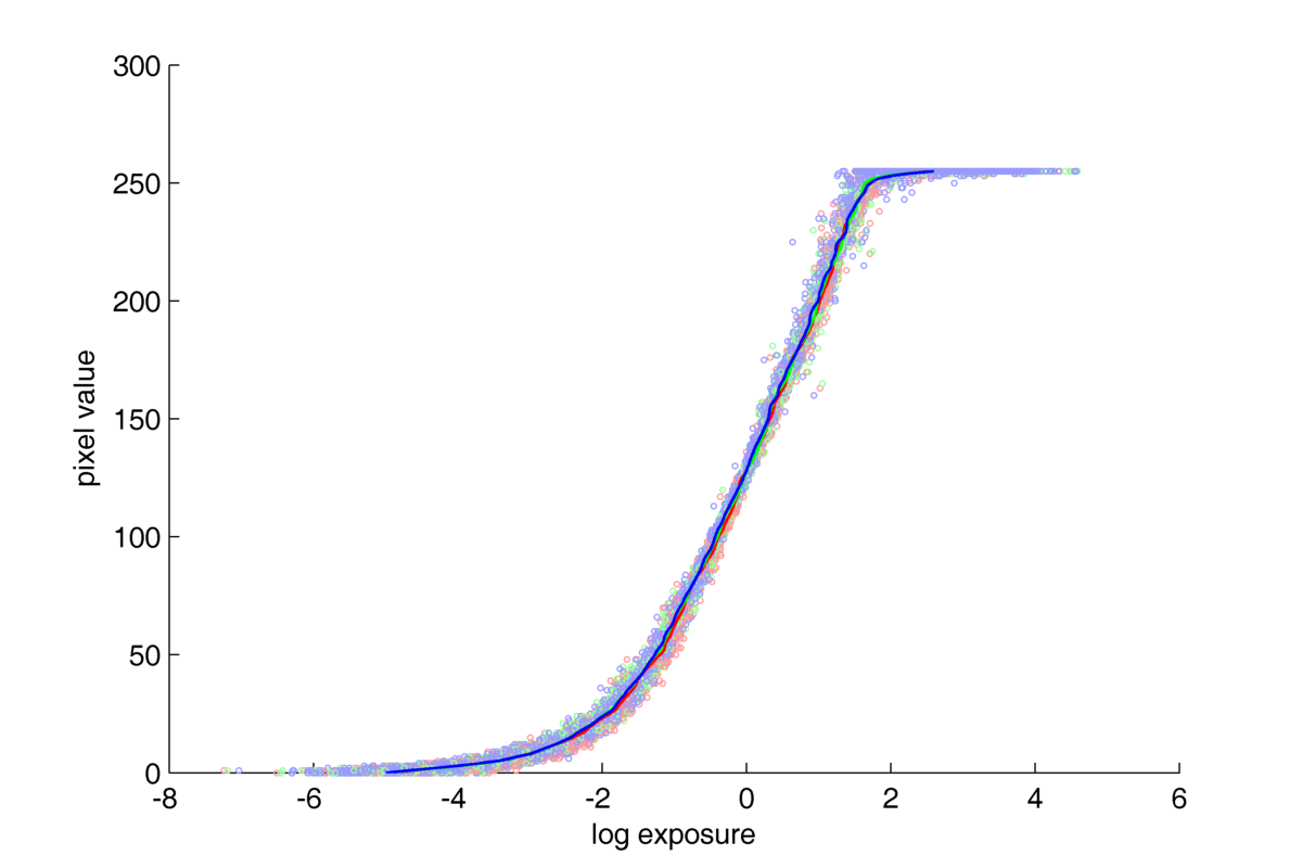
Nikon D70 response curve. NEF
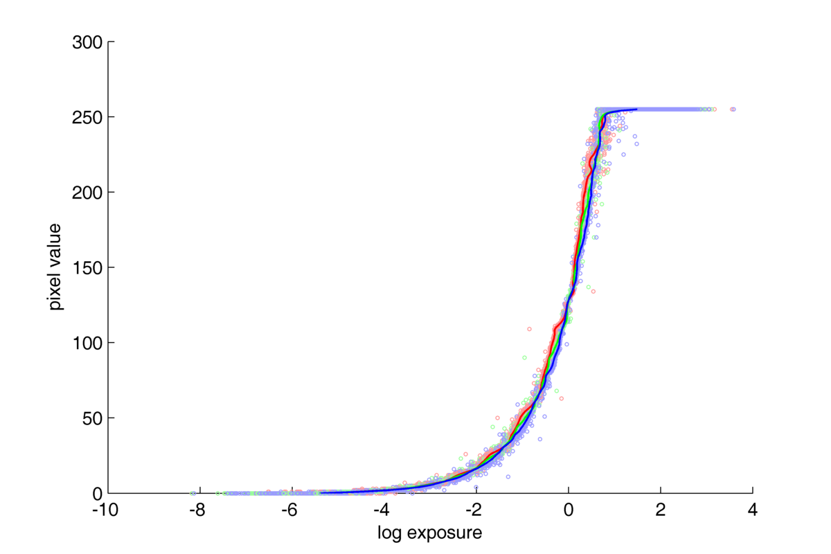
Nikon D70 response curve. NEF
We can observe that the response curve for NEF format has much more steep profile than the curve for JPG coding from previous article. But it is hard to tell more about differences between them as thay are both plotted here in semilog scale. To be able to compare them in more detail we have two options: plot them in the log-log scale, or in the linear-linear scale.
Plot with two axis linear for series 1:
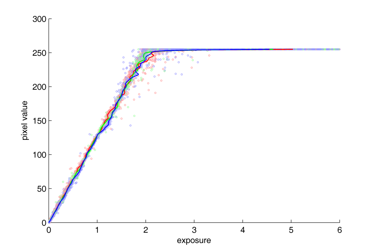
Nikon D70 response curve. NEF. lin-lin
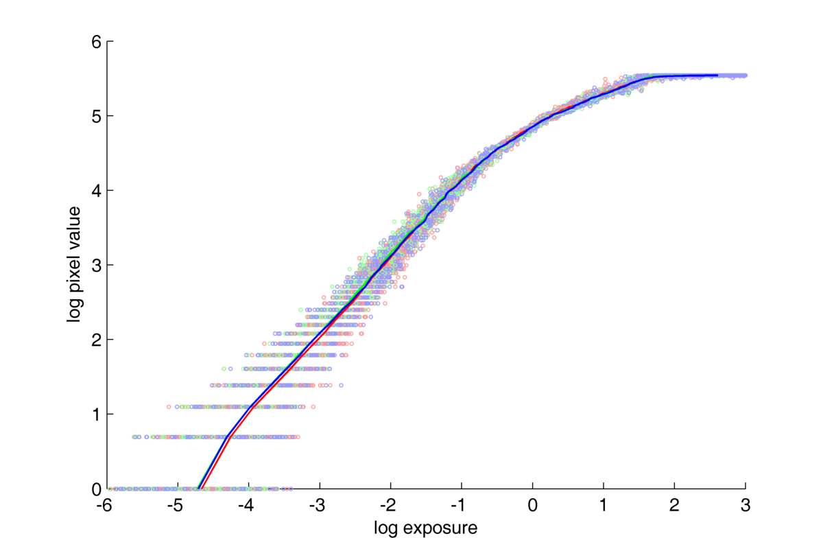
Plot with two axis logarythmic for series 1:
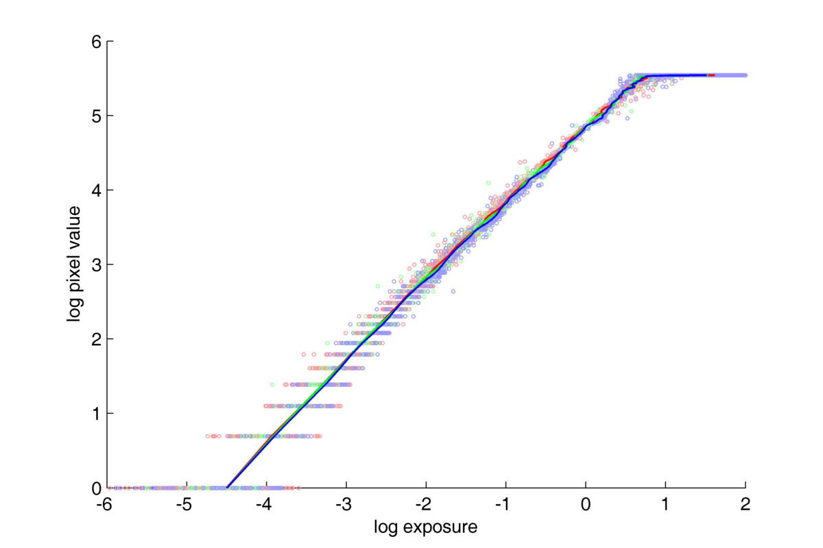
Nikon D70 response curve. NEF. log-log
In both these figures, the response function for NEF format is linear up to the range of saturation.
In the log-log plot, points localized in the bottom-left part of the space, can cause some serious concerns to the quality of the response curve estimation. The big dispersion of the points along X axis (logarythmioc exposure value) and big gaps between consequtive values along Y axis (logarythmic pixel value). The question of big gaps along Y axies becomes clear if we realize what exactly the transformation from linear to logarythmic scale does? The logarythmic scale makes the low values widely spread along axis, and keeps the higher ones more and more compressed. So, the big gaps between values in this region are the natural consequence of the tranformation of linear values into the logarythmic scale. We can evaluate, that in the half of the Y axis (in 0-3 range), there are exp(3)=20 pixels of all 256. Which means that in this scale, half of the space is taken by less than 8% of all possible pixel values. In the linear scale those values would take only a neglibly little space in the bottom-left corner of the plot. And the question of dispersion along X axis can be easily explained when taking under consideration the characteristic tendency of CCD sensors to register noise in low expositions, and the fact that half of the plot is taken by the 20 pixels for the lowest expositions. That is why, in the process of response curve estimation a weighting function, decreasing their weight in the calculations was used.
But what is the profile of the function for JPG formats in these scales?
Plot lin-lin:

Nikon D70 response curve. JPG. lin-lin
Plot log-log:
Nikon D70 response curve. JPG. log-log
On both of these plots, a nonlinear, gamma-like conversion can be observed.
Based on these both articles and presented results the conclusion about Nikon D70 can be made:
- saving pictures in JPEG format is associated with nonlinear transformation with profile presented on the plots above
- saving images in NEF format and flat conversion to 8-bit TIFFs by dcraw software, produces images with linear (in a certain range) response function.


 English
 polski